Recap
In the first post of this series, I walked through the basic ideas of what constitutes a graph, and in the second post I discussed a particular kind of graph called a directed acyclic graph (DAG), providing a handful of examples from the world of data engineering along with an attempt to disambiguate – and expand – the meaning of what a DAG is.
To briefly recap the important points discussed in this series so far:
- A graph consists of one or more nodes.
- Nodes are related to other nodes via one or more edges.
- Nodes that that can reach themselves again (in a single direction) indicate the graph has a cycle.
- A given edge can be directed or undirected.
- Nodes and edges can have attributes, including numerical attributes.
- Graphs without cycles, with only directed eges, are called directed acyclic graphs (DAGs).
- Hierarchies are DAGs in which each node only has a single predecessor node.
In the following post, we’re going to discuss hierarchies in detail. We’ll look at a few examples, discuss additional attributes that emerge from the definition of a hierarchy, and we’ll introduce an initial data model that can accommodate many different types of hierarchies.
Hierarchies
As indicated in the last post and summarized above, a hierarchy is essentially a DAG in which any given node has a single predecessor node (except for the root node, which has no predecessor). Given this constraint, predecessor nodes are most commonly referred to as “parent” nodes (i.e. with the analogy of a parent having one or more children). Successor nodes are thus also usually referred to as “child” nodes. We’ll stick with this convention for the rest of the series, given its wider adoption within BI vernacular.
(Note: despite the ideal case a hierarchy only ever consisting of child nodes with a single parent node, there are real-world edge cases where a given node can potentially have more than one parent node. Such cases are the exceptions, and they need to handled on a case-by-case basis. For our purposes, to manage scope of this overall series of posts, and in light of the expected cardinality of dimensional modeling (i.e. many-to-one from fact table to dimension tables), we’re going to move forward with the expectation that any/all hierarchies should always respect this relationship, i.e. a child node only ever having a single parent node.)
It’s also worth noting that hierarchies can be considered an instance of a “tree” data structure (a directed rooted tree, more specifically), which is a formally defined data structure from graph theory. While graph theory is rarely invoked in discussions of business intelligence, it is important to note that the tree analogy does indeed carry over, with terms like “root nodes”, “branches” and “leaf nodes” frequently used, which we’ll discuss later. (So just be mindful that you’re likely to run into mixed metaphors when discussing hierarchies.)
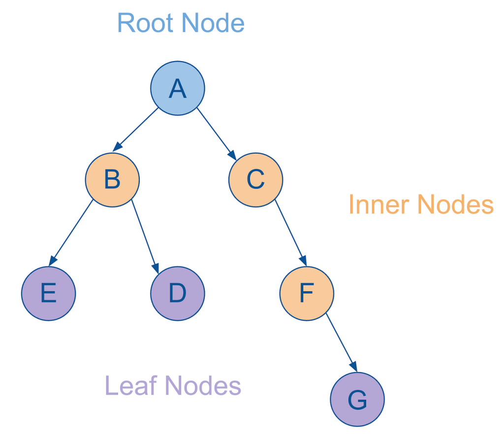
So, here’s a basic visualization of a hierarchy:
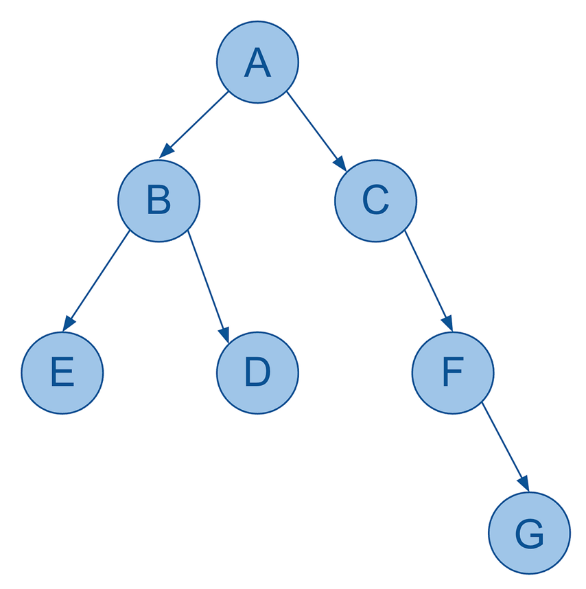
As you can see, it’s still very much a graph (and indeed a DAG) with:
- seven nodes
- six edges (directed)
- no cycles
- each node only has a single parent
So far so good.
I mentioned earlier that even though hierarchies have more constraints, i.e. they’re more limited in what they can represent compared to generic graphs, they nonetheless yield additional attributes. What do I mean by that?
Consider the following two points.
Firstly, because I have:
- a single starting point (i.e. the very first parent node),
- only directed edges,
- no cycles,
a hierarchy therefore allows me to measure the “distance” of any node in the hierarchy by how many edges away from the starting node (or “root node” as we’ll call it) it is. This measurement is typically referred to as which level a particular node is on (analogous to measuring how high up in a building you are by what level you’re on. And much like the British/American idiosyncracies around which floor constitutes the “first” floor, as well as the differences among programming languages regarding how arrays are indexed, i.e. starting at 0 or 1, you’ll also have to decide whether you index your root node at level 0 or 1. I don’t have a strong opinion and am guilty of having used both for no particular reason. I’ll try my best in these posts to arbitrarily stick with one convention, i.e. identifying the root node at level 1.)
Note that level is a value that can be derived from the data itself, and thus is slightly redundant when persisted as its own column – but such derivation introduces unnecessarily complex logic and performance headaches, and thus benefits from being persisted as part of transformation logic in a data pipeline.
Also note that this level attribute can be considered a node’s “natural” level, but that business requirements may dictate treating a node as though it has a different level. A more detailed discussion on such cases can be found in the 5th post of this series, where unbalanced and ragged hierarchies are addressed.
It’s also worth noting that you can, of course, measure the number of edges between any two nodes in a generic graph, but unlike with hierarchies, there’s not a single value for level per node but rather N-1 such values, i.e. since you can measure the number of edges between a given node and all other nodes in the same graph. Storing such information for all nodes introduce exponential storage requirements, i.e. O(n²), and offers very little technical or business value. Hence level is a fairly meaningless attribute in the context of generic graphs or DAGs.)
Secondly, because you can now refer to multiple “sibling” nodes under a single parent, you can describe the sort order of each sibling node. In other words, you define a particular sort order for all the related sibling nodes under a particular parent node. (This is another example of an attribute that is meaningful for hierarchies, but really doesn’t make much sense in the context of a generic graph or DAG.)
A classic example that demonstrates the value of a defined sort order attribute of hierarchy nodes are financial statements. (Just imagine in the following image of all of the lines were presented in a completely random order. It would make no sense at all.)
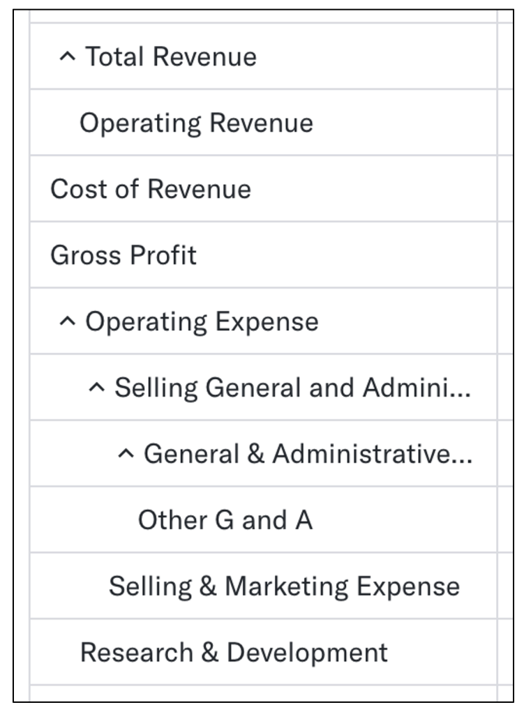
Financial reports are a very common use case in the world of BI, and it’s clearly extremely important to ensure that your reports display the various lines of your report in the correct order, defined by the sort order of each node in your financial statement hierarchy.
It’s worth noting that this sort order attribute doesn’t have a canonical name in the world of BI as such. But for a variety of reasons, my preference is “sequence number” (SEQNR as its column name), so we’ll stick with that. (Some data engineers / BI developers might refer to it as “ordinal position”, FYI).
(Also, for folks new to hierarchies, you might find it a worthwhile exercise to analyse the financial statement structure above as a hierarchy: How many nodes does it have? How many edges? How many levels? How many child nodes per parent? How might you actually model this data in a relational structure? We’ll come back to this in a bit.)
Two more points I’d like to make, as we work towards a generic/reusable data model for hierarchies:
- This should be obvious, but there are many different types of hierarchies, such as (in an enterprise context): profit centre hierarchies, cost centre hierarchies, WBS structure hierarchies, cost element hierarchies, financial statement hierarchies, and the list goes on.
- A particular hierarchy type might have multiple hierarchy instances. For example, a time dimension is actually a hierarchy, and almost all large enterprises care about tracking metrics along both the calendar year as well as the fiscal year, each of which is its own hierarchy.
And lastly, let me further extend the tree analogy introduced previously:
- As mentioned, the starting node is referred to as the root node.
- Any nodes that have parent and child nodes are called intermediate or inner nodes.
- Any nodes that have parent but no child nodes themselves are called leaf nodes.
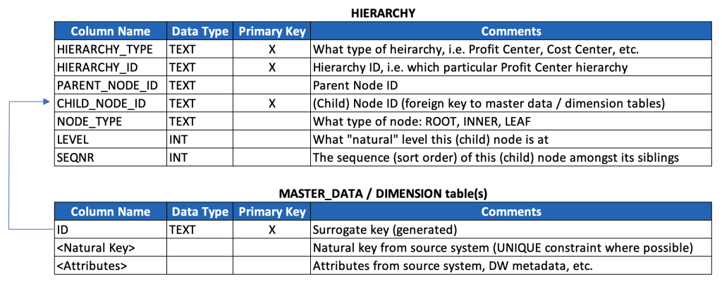
Ok, let’s now look at a basic, generic and reusable data model for storing hierarchies. This is the beginning of the discussion, and not the end, but it gives a strong foundation for how to accommodate many different types and instances of hierarchies.
Rather than write the SQL, I’m just going to provide a poor man’s data dictionary, especially given that your naming conventions (and probably also data types) may well differ. (For a detailed review of SQL that may help you ingest, model and consume hierarchies, see the 6th post in this series.)

Here below is what the example hierarchy above would look like in this model (key fields highlighted):

It’s worth taking a moment to talk through the model and the data a bit.
- This model denormalizes three levels of data: hierarchy types, hierarchy instances, and hierarchy nodes, and it also embeds a text description of hierarchy types (instead of a typical key/text pair). This is based on a pragmatic model that has been used successfully at multiple very large enterprises, but it’s worth considering whether your use case warrants a more normalized model. (And in either case, this model excludes separate language-dependent text tables that might be relevant if implementing a data model for a multinational organization, so just keep such tables in mind should you find yourself on such a project.)
- The primary key is a compound key based on these three levels. It’s worth noting that the CHILD_NODE_ID and HIERARCHY_ID should almost always be populated with generated surrogate keys, at least when data is ingested from multiple source systems. It’s also worth noting that it’s probably better to create a unique constraint against these three fields, and then generate a separate, single surrogate primary key (which will simplify later data modeling discussions). These details are left out from the above model for simplicity & illustration purposes.
- I’d suggest playing around a bit with some sample data, and sorting by the different columns, to familiarise yourself even more with this data model. For example, you could sort by NODE_TYPE to quickly find all the INNER nodes and LEAF nodes. You could sort by LEVEL and then SEQNR to “read” the hierarchy as you would with its visualised equivalent, i.e. top-to-bottom, left-to-right.
- Note that root nodes are defined as those records for which PARENT_NODE_ID is NULL. This is a commonly accepted convention, especially for query languages that can traverse parent-child hierarchies natively (such as MDX, which we’ll come back to), so I’d highly suggest adopting it (especially if you’re modeling in a strictly OLAP context), but there’s clearly no “formal” reason, i.e. from relational theory or anything else, that requires this.
- If this were a data model for a generic graph or even a DAG, we would have to include PARENT_NODE_ID as part of the primary key, since a node could have more than one parent. However, since hierarchy nodes only have a single parent node, we don’t need to do this, and in fact, we don’t want to do this (as, from a data quality perspective, it would let us insert records with multiple parent records, which breaks the definition set forth previously for hierarchies, and could lead to incorrect results in our BI queries by inflating metrics when joining hierarchies to fact tables due to M:N join cardinality instead of M:1).
- SEQNR values might be a bit confusing at first glance. While every row is populated a value, the values are only meaningful amongst sibling nodes. Also, note that the typical convention for populating SEQNR is to restart its numerical sequence for each set of siblings nodes, and thus values are often duplicated (i.e. re-used / reset for each set of sibling nodes).
- It’s technically possible to implement a contiguous sequence that spans all records, but that approach is usually avoided as it introduces another (arguably worse) form of confusion: it disregards the recursive relationship that exists between parent/child nodes.
- It’s also worth noting that in some cases, the only sort order that really matters is the inherent alphanumeric sort order (of the node IDs themselves, or their associated text descriptions), such as with the time dimension (so long as any alphanumeric representation is padded with zeroes so that the string “11” doesn’t appear before “2”, for example. For more on this, see the ISO 8601 standard.)
Before I forget to mention, you might hear this parent-child structure referred to as an “adjacency list”, which is another term from graph theory. Technically, an adjacency list maps a single node to all of its adjacent nodes within a single record (which could be accomplished by packing all adjacent nodes in an ARRAY or JSON data type). In practice though, folks often refer to the parent/child data model above as an adjacency list, even though each child node gets its own row. So just keep that in mind in case you hear folks use the term “adjacency list” somewhat casually.
Extending the Model
The basic hierarchy data model we’ve reviewed above can clearly accommodate multiple hierarchies of multiple different types, and after a bit of reflection it becomes obvious that each hierarchy type likely corresponds with its own dedicated master data and/or dimension with its own attributes.
So, we’ll extend our model with one additional generic table as a kind of placeholder for any/all dimensions that correspond with each hierarchy type that we’re persisting (keeping in mind that we may need to further extend the model to accommodate additional semantics around multilingual texts, currencies, units of measure, etc.).
In Summary
We’ve now gone through graphs, DAGs, and hierarchies, and we’ve walked through a basic, scalable data model for parent-child hierarchies and discussed some of the nuances of this model.
In the next post, we’ll review an alternative way to model hierarchies: the level hierarchy model. We’ll compare tradeoffs between parent-child and level hierarchy models, indicating when the level hierarchy might be more appropriate, and review a particularly helpful SQL query for “flattening” a parent-child hierarchy into a level hierarchy.
Epilogue – Disambiguation
After reviewing this series of posts as a whole, it occurred to me that it’s worth disambiguating various terms, concepts and conventions that I adopt throughout these posts to hopefully introduce a bit more clarity around the content of these posts but also the data engineering and BI industry more generally.
I also find myself taking a few shortcuts and liberties that fall short of academic rigor, that I think would be helpful to call out.
Hierarchies
- This series of posts is, primarily, about hierarchies found in business intelligence, i.e. data structures typically associated with dimensions that are used to aggregate KPIs/metrics at difference levels of granularity associated with the corresponding dimension. We could call these BI hierarchies.
- As noted in the beginning of this post, we’ve constrained BI hierarchies specifically to those that follow the strict definition of “directed root tree”, i.e. no multi-parent scenarios. It’s worth noting that there are many cases of data models and datasets that still meet this definition without strictly being treated as BI hierarchies, i.e. are made available for reporting without being specifically (or perhaps “frequently”) leveraged for rolling up / drilling down KPIs in a BI context, but nonetheless remain relevant data for reporting. We could call these technical hierarchies, i.e. data structures that meet the technical definition. (More on examples of such hierarchies discussed in the next post.)
- As noted in the prior post and next post (i.e. posts 2 and 4), there are many cases of data and/or capabilities in software that are called “hierarchical” without reference to BI, and without meeting the technical definition of a directed rooted tree.
- One example provided was the role-based access control (RBAC) of most databases. The structure of role inheritance makes it often, but not always, strictly hierarchical (i.e. given multi-parent inheritance as a possiblity).
- This is also true with time data (time dimension). Time data is very often used as a BI hierarchy, for drilling down and rolling up. But, this dimension/hierarchy is often modeled with week attributes, and if you think about, a calendar week can belong to more than one parent month, so casual use of “hierarchy” in the context of “month > week > day” relationships doesn’t quite meet the strict definition. I discuss this again in the next post.
The point here is not to over-analyze semantics, but rather just to indicate the latent ambiguity of language, in this case specifically regarding hierarchies. The best thing you can do is just stay mindful of context, and determine when specific senses/meanings of the term is intended. And the worst thing you can do is be dogmatic about a single definition and impost it in the wrong context.
This series of posts is primarily about BI hierarchies, but given some fascinating insights into more generic hierarchical data structures, I’ve decided to include additional content around what I’m calling “technical hierarchies” above. You’ll see what I mean in subsequent posts, and hopefully find the content interesting!
Parents and Children
We’ve discussed parent-child hierarchies, which may lead to some confusion when data modelers discuss “parent tables” and “child tables”. I find it helpful to recognize the following:
- A “child table” is a table that has a foreign key (whether formally or informally defined) that points back to the “parent table”, i.e. via its associated primary key.
- So, an ORDER table would be the parent of an ORDER_LINE table (and both could be fact tables used in different contexts, from a data warehousing perspective), and the join cardinality would be one-to-many.
- A supertype table (say a PERSON table) could be a parent table to multiple child tables (i.e. STUDENT table and FACULTY table). In this case, the join cardinality would be one-to-one (with the child tables storing records optionally, i.e. not all PERSON records have a corresponding CHILD table).
If you give it some thought, you’ll recognize that if you join any two such tables together, you’ll have a parent-child hierarchy (in the “technical” sense), i.e. the primary key of the parent table identifies the parent node, and the primary key of the child table identifies the child node. (Don’t get confused by composite keys, i.e. primary keys made up of multiple columns – just conceptually imagine concatenating them into a new column, so that you had a unique, single column key).
- The most common example would be typical dimension/fact table relationships. A single dimension record corresponds with multiple fact records (usually). Thus, if you consider just the dimension foreign key on the fact table (say, something like PRODUCT_ID) along with a generated primary key on your fact table (say FACT_ID), you then have a two-level hierarchy defined by PRODUCT_ID and FACT_ID. Thus, when you decide to aggregate metrics along that dimension, you are implicitly invoking the concept of a BI hierarchy, even if you have no further formal hierarchy levels in scope.
- Even in the case of super/subtype relationships, you also have a two-level hierarchy, where each parent node only has a single child node.
Disambiguating a few more things
- I tend to use “dimension” and “hierarchy” interchangeably when a dimension consists entirely of a hierarchy (such as with the time dimension itself – it’s a dimension, and it’s a hierarchy). Hopefully this is not confusing, as there are other cases where a single dimension (i.e. a PRODUCT dimension) consist of multiple (snowflaked) tables.
- On that note, I tend to use “snowflaking” and “normalizing” interchangeably.
- I tend to use “master data” and “dimension” interchangeably, since they both conceptually correspond with something representative of a single, well-understood entity. Obviously, master data tables from multiple source systems may be integrated into a single conformed dimension in an enterprise data warehouse, but I have a bad habit of nonetheless treating the terms as meaning more or less the same thing.
- When I use the word “structure” as a noun, it typically means “data model”, which I use whenever I use “model” as a verb. Otherwise “modeling a model” just sounds redundant/confusing.
And for reference, here are links to all of the posts in this series (next up is post #4):
Nodes, Edges and Graphs: Providing Context for Hierarchies (1 of 6)
More Than Pipelines: DAGs as Precursors to Hierarchies (2 of 6)
Family Matters: Introducing Parent-Child Hierarchies (3 of 6)
Flat Out: Introducing Level Hierarchies (4 of 6)
Edge Cases: Handling Ragged and Unbalanced Hierarchies (5 of 6)
Tied With A Bow: Wrapping Up the Hierarchy Discussion (Part 6 of 6)


