Tag: Data Analytics

The first five posts of these series were largely conceptual discussions that sprinkled in some SQL and data models here and there where helpful. This final post will serve as a summary of those posts, but it will also specifically include SQL queries, data models and transformation logic related to the overall discussion that should hopefully help you in your data engineering and analytics journey.

(Some of the content below has already been shared as-is, other content below iterates on what’s already been reviewed, and some is net new.)

And while this series of posts is specifically about hierarchies, I’m going to include SQL code for modeling graphs and DAGs as well just to help further cement the graph theory concepts undergirding hierarchies. As you’ll see, I’m going to evolve the SQL data model from one step to the next, so you can more easily see how a graph is instantiated as a DAG and then as a hierarchy.

I’m also going to use fairly generic SQL including with less commonly found features such as UNIQUE constraints. I’m certainly in the minority camp of Data Engineers that embrace the value offered by such traditional capabilities (which aren’t even supported in modern features such as Snowflake hybrid tables), and so while you’re unlikely to be able to implement some of the code directly as-is in a modern cloud data warehouse, they succinctly/clearly explain how the data model should function (and more practically indicate where you’ll need to keep data quality checks in mind in the context of your data pipelines, i.e. to basically check for what such constraints should be otherwise enforced).

And lastly, as alluded to in my last post, I’m not going to over-complicate the model. There are real-world situations that require modeling hierarchies either in a versioned approach or as slowly-changing dimensions, but to manage scope/complexity, and to encourage you to coordinate and learn from your resident Data Architect (specifically regarding the exact requirements of your use case), I’ll hold off on providing specific SQL models for such particularly complex cases. (If you’re a Data Architect reading this article, with such a use case on your hands, and you could use further assistance, you’re more than welcome to get in touch!)

Graphs 

Hierarchies are a subset of graphs, so it’s helpful to again summarize what graphs are, and discuss how they can be modeled in a relational database. 

A graph is essentially a data structure that captures a collection of things and their relationships to one another.

• A graph is also often referred to as a network.
• A “thing” is represented by a node in a graph, which is sometimes called a vertex in formal graph theory (and generally corresponds with an entity [i.e. a table] in relational databases, but can also correspond with an attribute [i.e. a column] of an entity).
• The relationship between two nodes is referred to as an edge, and two such nodes can have any number of edges.
• A node, quite obviously (as an entity) can have any number of attributes associated with it (including numerical attributes used in sophisticated graph algorithms [such as “biases” found in the graph structures of neural networks]).
• Oftentimes an edge is directed in a particular way (i.e. one of the nodes of the edge takes some kind of precedence over the other, such as in a geospatial sense, chronological sense, or some other logical sense).
• Edges often map to entities as well, and thus can have their own attributes. (Since LLMs are so popular these days, it’s perhaps worth pointing out how “weights” in neural networks are examples of numerical attributes associated with edges in a (very large) graph]).

Following is a basic data model representing how to store graph data in a relational database.

(It’s suggested you copy this code into your favorite text editor as .sql file for better formatting / syntax highlighting).

Modeling Graphs

Here is a basic data model for generic graphs. It consists of two tables:

• one for edges
• another for nodes (via a generic ENTITY table)

(It’s certainly possibly you’d also have a header GRAPH table that, at a minimum, would have a text description of what each graph represents. The GRAPH_ID below represents a foreign key to such a table. It’s not included here simply due to the fact that this model will evolve to support hierarchies which I usually denormalize such header description information directly on to.)

/*
    Graph nodes represent real world entities/dimensions.

    This is just a placeholder table for such entities, i.e.
    your real-world GRAPH_EDGE table would likely reference your master data/dimension 
    tables directly. 
*/
CREATE TABLE NODE_ENTITY
(
    ID INT,                    -- Technical primary key.
    ENTITY_ID_NAME,            -- Name of your natural key.
    ENTITY_ID_VALUE,           -- Value of your natural key.
    ENTITY_ATTRIBUTES VARIANT, -- Placeholder for all relevant attributes
    PRIMARY KEY (ID),
    UNIQUE(ENTITY_NAME, ENTITY_ID)
);

/*
    Graph edges with any relevant attributes. 

    Unique constraint included for data quality.
        - Multiple edges are supported in graphs
        - But something should distinguish one such edge from another.

    Technical primary key for simpler joins / foreign keys elsewhere.
*/
CREATE TABLE GRAPH_EDGE
(
    ID INT,                  -- Technical primary key (generated, i.e. by a SEQUENCE)
    GRAPH_ID INT,            -- Identifier for which graph this edge belongs to
    NODE_ID_1 INT NOT NULL,
    NODE_ID_2 INT NOT NULL,
    DIRECTION TEXT,          -- Optional. Valid values: FROM/TO. 
    EDGE_ID INT NOT NULL,    -- Unique identifier for each edge
    EDGE_ATTRIBUTES VARIANT, -- Placeholder for all relevant attributes
    -- constraints
    PRIMARY KEY (ID),
    UNIQUE (GRAPH_ID, EDGE_ID, NODE_1, NODE_2),
    FOREIGN KEY (NODE_ID_1) REFERENCES NODE_ENTITY (ID), 
    FOREIGN KEY (NODE_ID_2) REFERENCES NODE_ENTITY (ID), 
    CHECK (DIRECTION IN ('FROM', 'TO'))
);

DAGs

A directed acyclic graph, or DAG, represents a subset of graphs for which:

• Each edge is directed
• A given node cannot reach itself (i.e. traversing its edges in their respective directions will never return to node from which such a traversal started).

As such, a relational model should probably introduce three changes to accommodate the definition of a DAG:

• To simplify the model (and remove a potential data quality risk), it probably makes sense to remove the DIRECTION column and rename the node ID columns to NODE_FROM_ID and NODE_TO_ID (thereby capturing the edge direction through metadata, i.e. column names).
• The relational model doesn’t have a native way to constrain cycles, so a data quality check would need to be introduced to check for such circumstances.
• Technically, a DAG can have multiple edges between the same two nodes. Practically, this is rare, and thus more indicative of a data quality problem – so we’ll assume it’s reasonable to go ahead and remove that possibility from the model via a unique constraint (although you should confirm this decision in real life if you need to model DAGs.)

-- Renamed from GRAPH_EDGE
CREATE TABLE DAG_EDGE
(
    ID INT,
    DAG_ID,                    -- Renamed from GRAPH_ID                
    NODE_FROM_ID INT NOT NULL, -- Renamed from NODE_1
    NODE_TO_ID INT NOT NULL,   -- Renamed from NODE_2
    EDGE_ATTRIBUTES VARIANT,
    PRIMARY KEY (ID),
    UNIQUE (GRAPH_ID, NODE_1, NODE_2)
);

Hierarchies (Parent/Child)

A hierarchy is a DAG for which a given (child) node only has a single parent node (except for the root node, which obviously has no parent node). 

The concept of a hierarchy introduces a few particularly meaningful attributes (which have much less relevance to graphs/DAGs) that should be included in our model:

• LEVEL: How many edges there are between a given node and its corresponding root node, i.e. the “natural” level of this node.
  • This value can be derived recursively, so it need not strictly be persisted — but it can drastically simplify queries, data quality checks, etc.
• NODE_TYPE: Whether a given node is a root, inner or leaf node.
  • Again, this can be derived, but its direct inclusion can be incredibly helpful.
• SEQNR: The sort order of a set of “sibling” nodes at a given level of the hierarchy. 

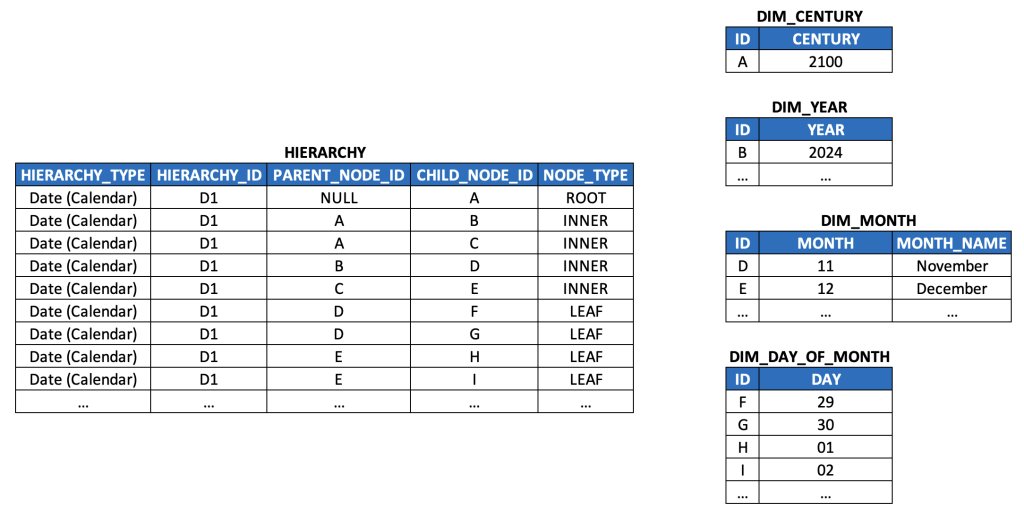
It’s also worth introducing a HIERARCHY_TYPE field to help disambiguate the different kind of hierarchies you might want to store (i.e. Profit Center, Cost Center, WBS, Org Chart, etc.). This isn’t strictly necessary if your HIERARCHY_ID values are globally unique, but practically speaking it lends a lot of functional value for modeling and end user consumption.

And lastly, we should rename a few fields to better reflect the semantic meaning of a hierarchy that distinguishes it from a DAG.

Note: the following model closely resembles the actual model I’ve successfully used in production at a large media & entertainment company for a BI use cases leveraging a variant of MDX.

-- Renamed from DAG_EDGE
CREATE TABLE HIERARCHY
(
    ID INT,              -- Technical primary key (generated, i.e. by a SEQUENCE) 
    HIERARCHY_TYPE TEXT, -- I.e. PROFIT_CENTER, COST_CENTER, etc.
    HIERARCHY_ID INT,    -- Renamed from DAG_ID
    PARENT_NODE_ID INT,  -- Renamed from NODE_FROM_ID
    CHILD_NODE_ID INT,   -- Renamed from NODE_TO_ID
    NODE_TYPE TEXT,      -- ROOT, INNER or LEAF
    LEVEL INT,           -- How many edges from root node to this node 
    SEQNR INT,           -- Ordering of this node compared to its siblings
    PRIMARY KEY (ID),
    UNIQUE (HIERARCHY_TYPE, HIERARCHY_ID, CHILD_NODE_ID)    
);

Now, it’s worth being a bit pedantic here just to clarify a few modeling decisions.

First of all, this table is a bit denormalized. In terms of its granularity, it denormalizes hierarchy nodes, with hierarchy instances, with hierarchy types. Thus, this table could be normalized out into at least 3 such tables. In practice, the juice just isn’t worth the squeeze for a whole variety of reasons (performance among them).

Also, to avoid confusion for end users, the traditional naming convention for relational tables (i.e. including the [singular] for what a given record represents) is foregone in favor of simply calling it just HIERARCHY. (Not only does this better map to user expectations, especially with a denormalized model, but also corresponds with the reality that we’re capturing a set of records that have a recursive relationship to one another, which in sum represent the structure of a hierarchy as a whole, and not just the individual edges.)

Hierarchies (Level)

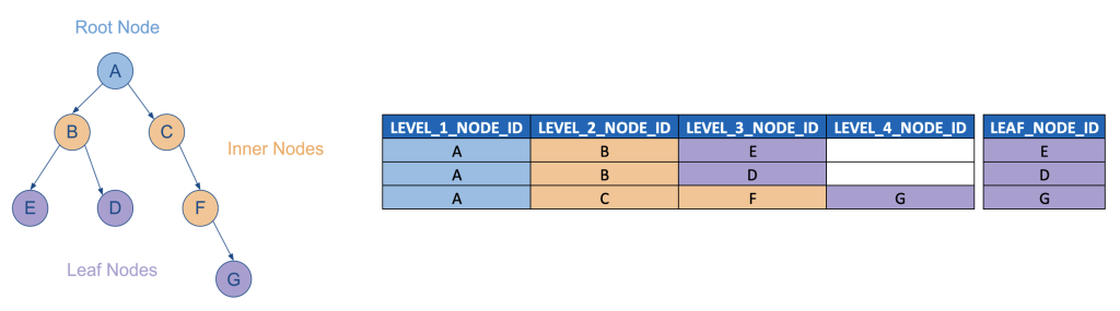
The parent/child model for hierarchies can be directly consumed by MDX, but given the prevalence of SQL as the query language of choice for “modern” BI tools and cloud data warehouses, it’s important to understand how to “flatten” a parent/child hierarchy, i.e. transform it into a level hierarchy.

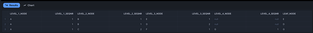
Such a level hierarchy has a dedicated column for each level (as well as identifying fields for the hierarchy type and ID, and also a dedicated LEAF_NODE column for joining to fact tables). The LEVEL attribute is represented in the metadata, i.e. the names of the columns themselves, and its important to also flatten the SEQNR column (and typically TEXT description columns as well).

(Remember that this model only reflects hierarchies for which fact table foreign keys always join to the leaf nodes of a given hierarchy. Fact table foreign keys that can join to inner nodes of a hierarchy are out of scope for this discussion.)

CREATE TABLE LEVEL_HIERARCHY
(
    ID INT,                  
    HIERARCHY_TYPE TEXT, 
    HIERARCHY_ID INT,    -- Renamed from DAG_ID. Often equivalent to ROOT_NODE_ID.
    HIERARCHY_TEXT TEXT, -- Often equivalent to ROOT_NODE_TEXT.
    ROOT_NODE_ID INT,    -- Level 0, but can be considered LEVEL 1.
    ROOT_NODE_TEXT TEXT,
    LEVEL_1_NODE_ID INT,
    LEVEL_1_NODE_TEXT TEXT,
    LEVEL_1_SEQNR TEXT,
    LEVEL_2_NODE_ID INT,
    LEVEL_2_NODE_TEXT TEXT,
    LEVEL_2_SEQNR TEXT,
    ...
    LEVEL_N_NODE_ID INT,
    LEVEL_N_NODE_TEXT TEXT,
    LEVEL_N_SEQNR TEXT,
    LEAF_NODE_ID           -- Joins to fact table on leaf node 
    PRIMARY KEY (ID),
    UNIQUE (HIERARCHY_TYPE, HIERARCHY_ID, LEAF_NODE_ID)    
);

Remember that level hierarchies come with the inherent challenge that they require a hard-coded structure (in terms of how many levels they represent) whereas a parent/child structure does not. As such, a Data Modeler/Architect has to make a decision about how to accommodate such data. 

• If some hierarchies are expected to rarely change, then a strict level hierarchy with the exact number of levels might be appropriate. 
• If other hierarchies change frequently (such as product hierarchies in certain retail spaces), then it makes sense to add additional levels to accommodate a certain amount of flexibility, and to then treat the empty values either as a ragged or unbalanced (see following sections below).
• Again, recall that some level of flexibility can be introduced by leveraging views in your consumption layer. One example of benefits of this approach is to project only those level columns applicable to a particular hierarchy / hierarchy instance, while the underlying table might persist many more to accommodate many different hierarchies.

Now, how does one go about flattening a parent/child hierarchy into a level hierarchy? There are different ways to do so, but here is one such way.

1. Use recursive logic to “flatten” all of the nodes along a given path into a JSON object.
2. Use hard-coded logic to parse out the nodes of each path at different levels into different columns. 

Here is sample logic, for a single hierarchy, that you can execute directly in Snowflake as is. 

(Given the unavoidable complexity of this flattening logic, I wanted to provide this code as is that readers can run directly without any real life data, so that they can immediately see the results of this logic in action.)

To extend this query to accommodate the models above, make sure you add joins HIERARCHY_ID and HIERARCHY_TYPE.

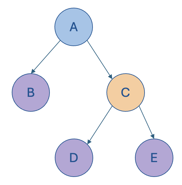
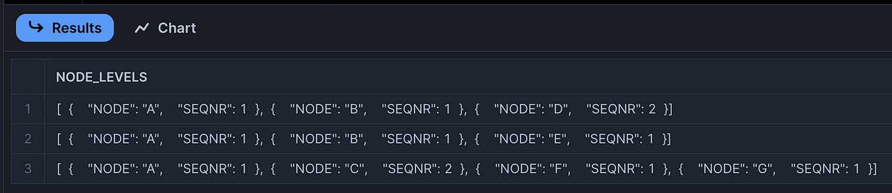
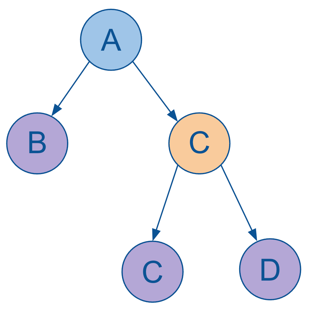
CREATE OR REPLACE VIEW V_FLATTEN_HIER AS
WITH 
    _cte_PARENT_CHILD_HIER AS 
    (
        SELECT NULL AS PARENT_NODE_ID, 'A' AS CHILD_NODE_ID, 0 AS SEQNR UNION ALL
        SELECT 'A' AS PARENT_NODE_ID, 'B' AS CHILD_NODE_ID, 1 AS SEQNR UNION ALL
        SELECT 'A' AS PARENT_NODE_ID, 'C' AS CHILD_NODE_ID, 2 AS SEQNR UNION ALL
        SELECT 'B' AS PARENT_NODE_ID, 'E' AS CHILD_NODE_ID, 1 AS SEQNR UNION ALL
        SELECT 'B' AS PARENT_NODE_ID, 'D' AS CHILD_NODE_ID, 2 AS SEQNR UNION ALL
        SELECT 'C' AS PARENT_NODE_ID, 'F' AS CHILD_NODE_ID, 1 AS SEQNR UNION ALL
        SELECT 'F' AS PARENT_NODE_ID, 'G' AS CHILD_NODE_ID, 1 AS SEQNR 
    )
    /*
        Here is the core recursive logic for traversing a parent-child hierarchy
        and flattening it into an array of JSON objects, which can then be further
        flattened out into a strict level hierarchy.
    */
    ,_cte_FLATTEN_HIER_INTO_OBJECT AS
    (
        -- Anchor query, starting at root nodes 
        SELECT 
            PARENT_NODE_ID,
            CHILD_NODE_ID, 
            SEQNR,
            -- Collect all of the ancestors of a given node in an array
            ARRAY_CONSTRUCT
            (
                /*
                    Pack together path of a given node to the root node (as an array of nodes) 
                    along with its related attributes, i.e. SEQNR, as a JSON object (element in the array)
                */
                OBJECT_CONSTRUCT
                (
                    'NODE', CHILD_NODE_ID, 
                    'SEQNR', SEQNR
                )
            ) AS NODE_LEVELS
        FROM 
            _cte_PARENT_CHILD_HIER
        WHERE 
            PARENT_NODE_ID IS NULL -- Root nodes defined as nodes with NULL parent
        
        UNION ALL
        
        -- Recursive part: continue down to next level of a given node
        SELECT             
            VH.PARENT_NODE_ID,
            VH.CHILD_NODE_ID, 
            CP.SEQNR,
            ARRAY_APPEND
            (
                CP.NODE_LEVELS, 
                OBJECT_CONSTRUCT
                (
                    'NODE', VH.CHILD_NODE_ID, 
                    'SEQNR', VH.SEQNR
                )
            ) AS NODE_LEVELS
        FROM 
            _cte_PARENT_CHILD_HIER VH
        JOIN 
            _cte_FLATTEN_HIER_INTO_OBJECT CP
        ON 
            VH.PARENT_NODE_ID = CP.CHILD_NODE_ID -- This is how we recursively traverse from one parent to its children
    )
    SELECT 
        NODE_LEVELS
    FROM 
        _cte_FLATTEN_HIER_INTO_OBJECT
    /*
        For most standard data models, fact table foreign keys for hierarchies only 
        correspond with leaf nodes. Hence filter down to leaf nodes, i.e. those nodes
        that themselves are not parents of any other nodes.
    */
    WHERE 
        NOT CHILD_NODE_ID IN (SELECT DISTINCT PARENT_NODE_ID FROM _cte_FLATTEN_HIER_INTO_OBJECT);

SELECT * FROM V_FLATTEN_HIER;

And then, to fully flatten out the JSON data into its respective columns: 

WITH CTE_LEVEL_HIER AS 
(
    /*
        Parse each value, from each JSON key, from each array element,
        in order to flatten out the nodes and their sequence numbers.
    */
    SELECT 
        CAST(NODE_LEVELS[0].NODE AS VARCHAR) AS LEVEL_1_NODE,
        CAST(NODE_LEVELS[0].SEQNR AS INT) AS LEVEL_1_SEQNR,
        CAST(NODE_LEVELS[1].NODE AS VARCHAR) AS LEVEL_2_NODE,
        CAST(NODE_LEVELS[1].SEQNR AS INT) AS LEVEL_2_SEQNR,
        CAST(NODE_LEVELS[2].NODE AS VARCHAR) AS LEVEL_3_NODE,
        CAST(NODE_LEVELS[2].SEQNR AS INT) AS LEVEL_3_SEQNR,
        CAST(NODE_LEVELS[3].NODE AS VARCHAR) AS LEVEL_4_NODE,
        CAST(NODE_LEVELS[3].SEQNR AS INT) AS LEVEL_4_SEQNR,
    FROM 
        V_FLATTEN_HIER
)
SELECT 
    *,
    /*
        Assuming fact records will always join to your hierarchy at their leaf nodes,
        make sure to collect all leaf nodes into a single column by traversing from
        the lower to the highest node along each path using coalesce() to find
        the first not-null value [i.e. this handles paths that reach different levels]/
    */
    COALESCE(LEVEL_4_NODE, LEVEL_3_NODE, LEVEL_2_NODE, LEVEL_1_NODE) AS LEAF_NODE
FROM 
    CTE_LEVEL_HIER
/*
    Just to keep things clean, sorted by each SEQNR from the top to the bottom
*/
ORDER BY 
    LEVEL_1_SEQNR,
    LEVEL_2_SEQNR,
    LEVEL_3_SEQNR,
    LEVEL_4_SEQNR;

Architecting your Data Pipeline

It’s clear that there are multiple points at which you might want to stage your data in an ELT pipeline for hierarchies:

• A version of your raw source data
• A parent/child structure that houses conformed/cleansed data for all of your hierarchies. This may benefit your pipeline even if not exposed to any MDX clients.
• An initial flattened structure that captures the hierarchy levels within a JSON object.
• The final level hierarchy structure that is exposed to SQL clients, i.e. BI tools.

A good question to ask is whether this data should be physically persisted (schema-on-write) or logically modeled (schema-on-read). Another good question to ask is whether any flattening logic should be modeled/persisted in source systems or your data warehouse/lakehouse.

The answers to these questions depend largely on data volumes, performance expectations, data velocity (how frequently hierarchies change), ELT/ETL standards and conventions, lineage requirements, data quality concerns, and your CI/CD pipelines compared to your data pipeline (i.e. understanding tradeoffs between metadata changes and data reloads).

So, without being overly prescriptive, here are a few considerations to keep in mind:

• For rarely changing hierarchies that source system owners are willing to model, a database view that performs all the flattening logic can often simplify extraction and load of source hierarchies into your target system. 
• For cases where logic cannot be staged in the source system, its recommended to physically persist copies of the source system data in your target system, aligned with typical ELT design standards. (In a majority of cases, OLTP data models are stored in parent/child structures.)
• Often times, OLTP models are lax with their constraints, i.e. hierarchies can have nodes with multiple parents. Such data quality risks must be addressed before exposing hierarchy models to end users (as multi-parent hierarchies will explode out metrics given the many-to-many join conditions they introduce when joined to fact tables).
• Different hierarchy types often have very different numbers of levels, but obviously follow the same generic structure within a level hierarchy. As such, it likely makes sense to physically persist the structure modeled in the V_FLATTEN_HIER view above, as this model supports straightforward ingestion of hierarchies with arbtirary numbers of levels. 
• For particular hierarchy instances that should be modeled in the consumption layer, i.e. for BI reporting, it’s worth considering whether you can get sufficiently good performance from logical views that transform the JSON structure into actual columns. If not, then it may be worth physically persisting a table with the maximum required number of columns, and then exposing views on top of such a table that only project the required columns (with filters on the respective hierarchies that are being exposed). And then, if performance still suffers, obviously each hierarchy or hierarchy type could be persisted in its own table. 

Ragged and Unbalanced Hierarchies

You may or may not need to make any changes to your parent/child data model to accommodate ragged and unbalanced hierarchies, depending on whether or not that structure is exposed to clients.

Given the rare need for MDX support these days, it’s probably out of scope to flesh out all of the details of the modeling approaches already discussed, but we can at least touch on them briefly:

1. The primary issue is capturing the correct LEVEL for a given node if it differs from its “natural” level reflected natively in the hierarchy. If there’s relatively few such exceptional cases, and they rarely change, then the best thing to do (most likely) would be to add an additional column called something like BUSINESS_LEVEL to capture the level reflected in the actual business / business process that the hierarchy models. (I would still recommend maintaining the “natural” LEVEL attribute for the purposes of risk mitigation, i.e. associated with data quality investigations.)
2. Otherwise, for any more complex cases, it’s worth considering whether it makes sense to introduce a bridge table between your hierarchy table and your node table, which captures either different version, or history, of level change over time. (Again, such versioning as well as “time dependency” could really make sense on any of the tables in scope – whether this proposed bridge table, the hierarchy table itself, the respective node entity tables, and/or other tables such as role-playing tables.)

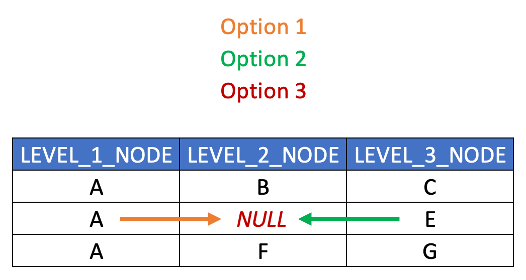
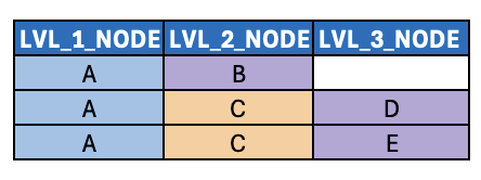
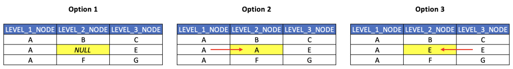
In terms of handling ragged hierarchies in a level structure, the typical approach is to “extrapolate” either the nearest ancestor or the nearest descendant nodes, or to populate the empty nodes with NULL or a placeholder value. Here below is a simplified visualization of such approaches. Ensure your solutions aligns with end user expectations. (The SQL required for this transformation is quite simple and thus isn’t explicitly included here.)

Note that relaated columns are absent from this example just for illustration purposes (such as HIERARCHY_ID, SEQNR, TEXT and LEAF_NODE columns.)

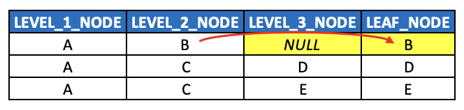
And lastly, in terms of handling unbalanced hierarchies in a level structure, the typical approach is:

1. As with all level hierarchies, extrapolate leaf node values (regardless of what level they’re at) into a dedicated LEAD_NODE column (or LEAF_NODE_ID column), and
2. Populate the empty level columns with either NULL or PLACEHOLDER values, or potentially extrapolate the nearest ancestor values down through the empty levels (if business requirements dictate as much).

Note that required columns are absent from this example just for illustration purposes (such as HIERARCHY_ID, SEQNR and TEXT columns.)

Concluding Thoughts

Over the course of this series, we’ve covered quite a bit of ground when it comes to hierarchies (primarily, but not exclusively, in the context of BI and data warehousing), from their foundational principles to practical data modeling approaches. We started our discussion by introducing graphs and directed acyclic graphs (DAGs) as the theoretical basis for understanding hierarchies, and we built upon those concepts by exploring parent-child hierarchies, level hierarchies, and the tradeoffs between them.

As a consequence, we’ve developed a fairly robust mental model for how hierarchies function in data modeling, how they are structured in relational databases, and how they can be consumed effectively in BI reporting. We’ve also examined edge cases like ragged and unbalanced hierarchies, heterogeneous hierarchies, and time-dependent (slowly changing dimension) and versioned hierarchies, ensuring that some of the more complex concepts are explored in at least some detail.

Key Takeaways

To summarize some of the most important insights from this series:

1. Hierarchies as Graphs – Hierarchies are best conceptualized as a subset of DAGs, which themselves are a subset of graphs. Understanding how to models graphs and DAGs makes it easier to understand how to model hierarchies (including additional attributes such as LEVEL and SEQNR).
2. Modeling Hierarchies – There are two primary modeling approaches when it comes to hierarchies: parent-child and level hierarchy models. The flexibility/reusability of parent-child hierarchies lends itself to the integration layer whereas level hierarchies lend themselves to the consumption layer of a data platform/lakehouse.
3. Flattening Hierarchies – Transforming parent-child hierarchies to level hierarchies (i.e. “flattening” hierarchies) can be accomplished in several ways. The best approach is typically via recursive CTEs, which should be considered an essential skills for Data Engineers.
4. Hierarchies Are Everywhere – Hierarchies, whether explicit or implicit, can be found in many different real-world datasets, and many modern file formats and storage technologies are modeled on hierarchical structures and navigation paths including JSON, XML and YAML. Hierarchies also explain the organization structure of most modern file systems.
5. Hierarchy Design Must Align with Business Needs – Theoretical correctness means little if it doesn’t support practical use cases. Whether modeling financial statements, org charts or product dimensions, hierarchies should be modeled, evolved and exposed in a fashion that best aligns with business requirements.

I genuinely hope this series has advanced your understanding and skills when it comes to hierarchies in the context of data engineering, and if you find yourself with any lingering questions or concerns, don’t hesitate to get in touch! LinkedIn is as easy as anything else for connecting.

In the first three posts of this series, we delved into some necessary details from graph theory, reviewed acyclic graphs (DAGs), and touched on some foundational concepts that help describe what hierarchies are and how they might best be modeled. 

In the fourth post of the series, we spent time considering an alternative model for hierarchies: the level hierarchy which motivated several interesting discussion points including:

• The fact that many common fields (and collections of fields) in data models (such as dates, names, phone numbers, addresses and URLs) actually encapsulate level hierarchies.

• A parent-child structure, as simple/robust/scalable as it can be, can nonetheless overcomplicate the modeling of certain types of hierarchies (i.e. time dimensions as a primary example).

• Level hierarchies are also the requisite model for most “modern data stack” architectures (given that a majority of BI tools do not support native SQL-based traversal of parent-child hierarchies).

• As such, parent-child hierarchies are often appropriate for the integration layer of your data architecture, whereas level hierarchies are often ideal for your consumption layer.
  • The corresponding “flattening” transformation logic should probably be implemented via recursive CTEs (although other approaches are possible, such as self-joins).
  • When/where to model various transformations, i.e. in physical persistence (schema-on-write) or via logical views (schema-on-read), and at what layer of your architecture depends on a number of tradeoffs and should be addressed deliberately with the support of an experienced data architect.

At the very end of the last (fourth) post, we examined an org chart hierarchy that included a node with a rather ambiguous level attribute. The “natural” level differed from the “business” level and thus requires some kind of resolution.

So, let’s pick back up from there. 

Introducing Unbalanced & Ragged Hierarchies

Unbalanced Hierarchies

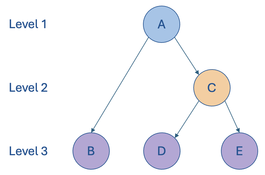
We had a quick glance at this example hierarchy, which is referred to as an unbalanced hierarchy:

• In this example, node B is clearly a leaf node at level 2, whereas the other leaf nodes are at level 3.
• Stated differently, not all paths (i.e. from the root node to the leaf nodes) extend to the same depth, hence giving this model the description of being “unbalanced”.

As we indicated previously, most joins from fact tables to hierarchies take place at the leaf nodes. Given the unbalanced hierarchies have leaf nodes at different levels, there’s clearly a challenge in how to effectively model joins against fact tables in a way that isn’t unreasonably brittle.

We did solve for this particularly challenge (by introducing a dedicated leaf node column, i.e. LEAF_NODE_ID), but there are more to consider later on.

But let’s next introduce ragged hierarchies.

Ragged Hierarchies

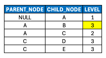
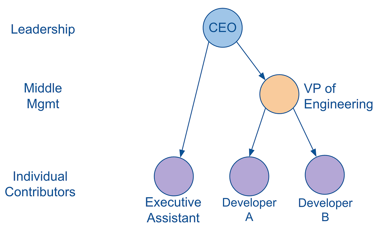
In the last post, we provided a concrete example of this hierarchy as an org chart, demonstrating how node B (which we considered as an Executive Assistant in a sample org chart) could be described as having a “business” level i.e. of 3 that differs from what we’re calling its “natural” level of 2. We’ll refer to such hierarchies as ragged hierarchies.

(For our purposes, we’ll only refer to the abstract version of the hierarchy for the rest of this post, but it’s worth keeping real-world use cases of ragged hierarchies in mind, such as the org chart example.)

A ragged hierarchy is defined as a hierarchy in which at least one parent node has a child node specified at more than one level away from it. So in the example above, node B is two levels away from its parent A. This also means that ragged hierarchies contain edges that span more than one level (i.e. the edge [A, B] spans 2 levels).

Ragged hierarchies have some interesting properties as you can see. For example:

• Adjacent leaf nodes might not be sibling nodes (as is the case with nodes B and D).
• Sibling nodes can be persisted at different (business) levels, i.e. nodes B and C.

The challenge with ragged hierarchies is trying to meaningfully aggregate metrics along paths that simply don’t have nodes at certain levels.

Having now introduced unbalanced and ragged hierarchies, let’s turn out attention to how to model them in parent-child and level hierarchy structures.

Modeling Unbalanced and Ragged Hierarchies

Modeling Unbalanced Hierarchies (Parent/Child)

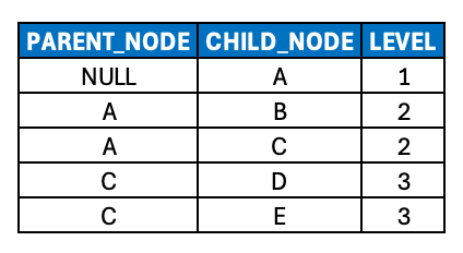
A parent/child structure lends itself to directly modeling an unbalanced hierarchy. The LEVEL attribute corresponds directly to the derived value, i.e. the “depth” of a given node from the root node. (It’s also worth noting that B, despite being a leaf node at a different level than other leaf nodes, is still present in the CHILD_NODE column as with all leaf nodes, supporting direct joins to fact tables (and/or “cubes”) in the case of MDX or similar languages).

No specific modifications to either the model or the data are required.

• No modifications need if you’re querying this data with MDX from your consumption layer.
• No modifications needed if you model this data in your integration layer (i.e. in a SQL context).
  • But as already discussed, if SQL is your front-end’s query language (most likely), then of course this model won’t serve well in your consumption layer.

Modeling Unbalanced Hierarchies (Level)

With the assumption previously discussed that any/all related fact tables contain foreign key values only of leaf nodes of a given hierarchy, node B should be extended into the dedicated LEAF_NODE (or LEAF_NODE_ID depending on your naming conventions) column introduced in the last post (along with nodes D and E). Thus, joins to fact tables can take place consistently against a single column, decoupled from the unbalanced hierarchy itself.

The next question, then, becomes – what value should be populated in the LEVEL_3_NODE column?

Generally speaking, it should probably contain NULL or some kind of PLACEHOLDER value. That way, the resulting analytics still show metrics assigned to node B (via the leaf node join), but they don’t roll up to a specific node value at level 3, since none exists. Then at LEVEL_2_NODE aggregations, the analytics clearly show the LEAF_NODE value matching LEVEL_2_NODE. 

(For illustration purposes, I’m leaving out related columns such as SEQNR columns)

Another option is to also extend the leaf node value, i.e. B, down to the missing level (i.e. LEVEL_3_NODE).

• This approach basically transforms an unbalanced hierarchy into a ragged hierarchy. It’s a less common approach, so it’s not illustrated here.

Modeling Ragged Hierarchies (Parent/Child)

A parent/child structure can reflect a ragged hierarchy by modeling the data in such a way that the consumption layer queries the business level rather than the natural level. The simplest way to do so would be to just modify your data pipeline with hard-coded logic to modify the nodes in question by replacing the natural level with the business level, as visualized here. (Note that this could done physically, i.e. as data is persisted in your pipeline, or logically/virtually in a downstream SQL view.)

Such an approach might be okay if:

• such edge case (nodes) are rare
• if the hierarchies change infrequently,
• if future changes can be managed in a deliberate fashion,
• and if it’s very unlikely that any other level attributes need to be managed (i.e. more than one such business level)

Otherwise, this model is likely to be brittle and be difficult to maintain, in which case the integration layer model should probably be physically modified to accommodate multiple different levels, and the consumption layer should also be modified (whether physically or logically) to ensure the correct level attribute (whether “natural”, “business” or otherwise) is exposed. This is discussed in more detail below in the section “Versioning Hierarchies”.

Modeling Ragged Hierarchies (Level)

Assuming the simple case described above (i.e. few number of edge case nodes, infrequent hierarchy changes), ragged hierarchies can be accommodated in 3 ways, depending on business requirements:

1. Adding NULL or a PLACEHOLDER value at the missing level,
2. Extending the parent node (or nearest ancestor node, more precisely) down to this level (this is the most common approach),
3. Or extending the child node (or nearest descendant node) up to this level.

A final point worth considering is that it’s technically possible to have a hierarchy that is both unbalanced and ragged. I’ve never seen such a situation in real-life, so I’ll leave such an example as an exercise to the reader. Nonetheless, resolving such an example can still be achieved with the approaches above.

Versioning Hierarchies

As mentioned above, real-life circumstances could require a data model that accommodates multiple level attributes (i.e. in the case of ragged hierachies, or in the case of unbalanced hierarchies that should be transformed to ragged hierarchies for business purposes). There are different ways to do so.

• We could modify our hierarchy model with additional LEVEL columns. This approach is likely to be both brittle (by being tightly coupled to data that could change) and confusing (by modifying a data-agnostic model to accommodate specific edge cases). This approach is thus generally not recommended.
• A single additional semi-structured column, i.e. of JSON or similar type, would more flexibly accommodate multiple column levels but can introduce data quality / integrity concerns.

(At the risk of making this discussion more confusing that it perhaps already is, I did want to note that there could be other reasons (beyond the need for additional level attributes) to maintain multiple versions of the same hierarchy, which further motivate the two modeling approaches below. For example, in an org chart for a large consulting company, it’s very common for consultants to have a line (reporting) manager, but also a mentor, and then also project managers. So depending on context, the org chart might slightly different in terms of individual parent/child relationships, which often is considered a different version of the same overarching hierarchy.)

1. Slowly-changing dimensions (hierarchies) – Using the org chart example, it’s clearly possible that an Executive Assistant to a CEO of a Fortune 100 company is likely higher on an org chart than an Executive Assistant to the CEO of a startup. As such, it’s quite possible that their respective level changes over time as the company grows, which can be captured as a slowly changing dimension, i.e. type 2 (or apparently type 7 as Wikipedia formally classifies it).
   • Keep in mind these changes could be to the hierarchy itself, the employee themselves, the role they’re playing at given points in time, and/or some instantiation of the relationship between any of these two (or other) entities. Org chart data models can clearly get quite complicated.
2. Versioned dimensions – I don’t think “versioned dimensions” is a formal term in data engineering, but it’s helpful for me at least to conceptualize a scenario where different use cases leverage the exact same hierarchy with slight changes, i.e. one use case (such as payroll analytics) considering the ragged hierarchy version, whereas another use case (such as equity analytics) considering the unbalanced version. Such situations would warrant a versioning bridge table (between the hierarchy table and the HR master data / dimension table, for example) that consists of at least four (conceptual) columns: a foreign key point to the hierarchy table, a foreign key pointing to the dimension table, a version field (i.e. an incrementing integer value for each version), and the LEVEL field with its various values depending on version. (A text description of each version would clealy also be very helpful.)
   • Keep in mind that such versioning could be accomplished by physically persisting only those nodes that have different versions, or physically persisting all nodes in the hierarchy.
     • Performance plays a role in this decision, depending on how consumption queries are generated/constructed (and against what data volumes, with what compute/memory/etc.)
     • Clarity also plays a role. If 80% of nodes can have multiple versions, for example, I would probably recommend completely persisting the entire hierarchy (i.e. all of the corresponding nodes) rather than just the nodes in question.

For the time being, I’ll hold off on providing actual SQL and data models for such data model extensions. I want to help bring awareness to readers on ways to extend/scale hierarchy data models and demonstrate where some of the complexities lie, but given how nuanced such cases can end up, I’d prefer to keep the discussion conceptual/logical and hold off on physical implementation (while encouraging readers to coordinate closely with their respective Data Architect when encountering such scenarios).

This particular omission notwithstanding, the next and final post will summarize these first five points and walk through the corresponding SQL (data models and transformation logic) to help readers put all of the concepts learned thus far into practice.

And for reference, here are links to all of the posts in this series (next up is the final post #6):

Nodes, Edges and Graphs: Providing Context for Hierarchies (1 of 6)

More Than Pipelines: DAGs as Precursors to Hierarchies (2 of 6)

Family Matters: Introducing Parent-Child Hierarchies (3 of 6)

Flat Out: Introducing Level Hierarchies (4 of 6)

Edge Cases: Handling Ragged and Unbalanced Hierarchies (5 of 6)

Tied With A Bow: Wrapping Up the Hierarchy Discussion (Part 6 of 6)

In the first post of this series, we walked through the basic concepts of a graph. In the second post, we discussed a particular kind of graph called a directed acyclic graph (DAG) and helped disambiguate and extend the roles it plays in data engineering. In the third post, we further constrained the definition of a DAG to arrive at the definition of a hierarchy and introduced some basic terminology along with a generic parent-child data model for hierarchies. 

To briefly recap the important points from those first three posts:

• A graph consists of one or more nodes connected by one or more edges.

• Nodes and edges can have various attributes associated with them, including numerical attributes.

• Direct, acyclic graphs (DAGs) consist only of graphs with directed edges, without cycles (i.e. nodes cannot reach themselves when traversing the graph in the direction of the edges.)

• Hierarchies are DAGs in which each node has only a single predecessor node.

• Hierarchy nodes are often characterized by the analogy of a family, in which a given parent (predecessor) node can have multiple child (successor) nodes. The analogy also includes intuitive concepts of sibling nodes, ancestor nodes and descendant nodes.

• Hierarchy nodes are also characterized by the analogy of a tree, in which the first parent node in a hierarchy is called a root node, the terminal child nodes in a hierarchy are called leaf nodes, and all nodes between the root node and leaf nodes are called inner (or intermediate) nodes.

• It’s helpful to track two additional attributes for hierarchy nodes. The first attribute is the sequence number, which defines the sort order amongst a set of sibling nodes. The second attribute is the level, which generally describes how many edges a given node is removed from the root node.

• Hierarchies can be modeled in a parent-child structure, also colloquially referred to as adjacency list, which can be extended to accommodate multiple instances of multiple types of hierarchies.

In this fourth post, we’re going to introduce an alternative data model: the level hierarchy data model. We’ll discuss cases when this model is more helpful than a parent-child hierarchy, and we’ll review SQL logic that can be used to “flatten” a parent-child hierarchy into a level hierarchy.

Level Hierarchies

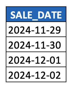
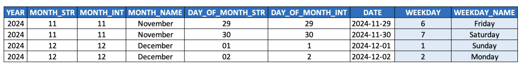
In the last post, I made reference to the time dimension. It’s the first type of dimension introduced in an academic context, it’s usually the the most important dimension in data warehouse models, and it’s well-suited for modeling as a level hierarchy. So, let’s start our discussion there. And just for fun, let’s start by looking at a simple DATE column, because it actually corresponds with a (level) hierarchy itself.

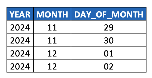
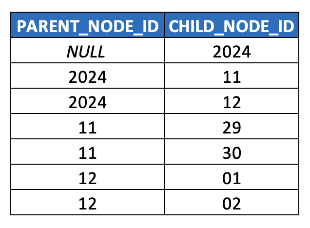
Such DATE values are really nothing more than hyphen-delimited paths across three levels of a time hierarchy, i.e. YEAR > MONTH > DAY. To make this picture more explicit, parsing out the individual components of a DATE column generates our first example of a level hierarchy:

In terms of considering this data as a hierarchy, it quickly becomes obvious that:

• The first column YEAR represents the root node of the hierarchy,

• Multiple DAY_OF_MONTH values roll up to a single MONTH value, and multiple MONTH values roll up to a single YEAR value
  • i.e. multiple child nodes roll up to a single parent node

• Any two adjacent columns reflect a parent-child relationship (i.e. [YEAR, MONTH] and [MONTH, DAY_OF_MONTH]),
  • So we could think of this is as parent-child-grandchild hierarchy table, i.e. a 3-level hierarchy
  • Clearly this model could accommodate additional ancestor/descendant levels (i.e. if this data were stored as a TIMESTAMP, it could also accommodate HOUR, MINUTE, SECOND, MILLISECOND, and NANOSECOND levels).

• Each column captures all nodes at a given level (hence the name “level hierarchy”), and

• Each row thus represents the path from the root node all the way down to a given leaf node (vs. a row in a parent-child model which represent a single edge from a parent node to a child node).
  • Thus, one consequence of level hierarchies is that ancestor nodes are duplicated whenever there are sibling nodes (i.e. more than one descendant node at a given level) further along any of its respective paths. You can see above how YEAR and MONTH values are duplicated. This duplication can impact modeling decisions when measures are involved. More on this later.)
    • Duplication of parent nodes can obviously occur in a parent-child hierarchy, but this doesn’t pose a problem since joins to fact tables are always on the child node column.

(Note in the example above that I took a very common date field, i.e. SALE_DATE, just to illustrate the concepts above. In a real-world scenario, SALE_DATE would be modeled on a fact table, whereas this post is primary about the time dimension (hierarchy) as a dimension table. This example was not meant to introduce any confusion between fact tables and dimension tables, and as noted below, a DATE field would be persisted on the time dimension and used as the join key to SALE_DATE on the fact table.)

Side Note 1

Keep in mind that in a real-world time dimension, the above level hierarchy would also explicitly maintain the DATE column as well (i.e. as its leaf node), since that’s the typical join key on fact tables. As such, the granularity is at the level of dates rather than days, which might sound pedantic, but from a data modeling perspective is a meaningful distinction (a date being an instance of a day, i.e. 11/29/2024 being an instance* of the more generic 11/29). This also avoids the “multi-parent” problem that a given day (say 11/29) actually rolls up to all years in scope (which again is a trivial problem since very few fact tables would ever join on a month/year column).

It’s also worth noting that this means the level hierarchy above technically represents multiple hierarchies (also called “subtress” or sometime sub-hierarchies) if we only maintain YEAR as the root node. This won’t cause us any problems in practice assuming we maintain the DATE column (since such leaf nodes aren’t repeated across these different sub-hierarchies, i.e. a given date only belongs to a given year). Do be mindful though with other hierarchy types where the same leaf node could be found in multiple hierarchies (i.e. profit centre hierarchies as one such example): such scenarios require some kind of filtering logic (typically prompting the user in the UI of the BI tool to select which hierarchy they want to consider in their dashboard/report) to ensure leaf values aren’t inadvertently duplicated.

*From a data modeling perspective, it’s worth reflecting on when you’re modeling instances of things versus classes of things. As mentioned, in the case of a time dimension, a date is a specific instance of a more generic “day” concept (class). Time dimensions are part of most retail data models, which have two additional dimensions that highlight the distinction between instances and classes. The product dimension, for example is typically modeled as classes of products (i.e. a single record might represent all iPhones of a specific configuration), whereas store dimensions are typically modeled as specific store instances.

This distinction between classes/instances is analogous to classes/objects in object-oriented programming, although a programming “object” (instance of a Java class, for example) can certainly represent a real-world class (i.e. the class of all iPhone 15 Pro Max phones). What’s less common is a “class” in an OO language representing a real-world object (i.e. instance).

Side Note 2

As indicated above, the time dimension level hierarchy can clearly be extended to higher and lower levels if/as needed depending on use case. As on example, event data is often captured at the level of TIMESTAMP, whether at the second, millisecond ,or possibly nanosecond level. And in cases of scientific research, i.e. in fields like astronomy or particle physics (not impossible – apparently CERN produces massive amounts of data), there is actually occasion to extend this model particularly far at one end or the other.

Granted, I doubt scientific researchers are using relational/dimensional models and technology for their analysis, but it makes for a fun thought experiment. Apparently it would only take about 60 columns to model the age of the universe down to Planck units if you really wanted to, which is obviously ridiculous but a fun thought experiment. But according to ChatGPT, storage of this data even in a medium as dense as DNA would still exceed the known mass of the universe!)

Side Note 3

Given that a DATE column can be understood as a compact representation of a hierarchy, I find it personally insightful to keep an eye out for similar cases, i.e. instances of structured data representing more complex structures (i.e. hierarchies) even when not explicitly modeled as such.

For example:

• Tables that contain FIRST_NAME and LAST_NAME indicate an implicit (and quite literal) parent-child hierarchical structure of family members and families.

• Address fields such as STREET_NAME, STREET NUMBER, POSTAL_CODE, CITY, COUNTRY, etc. reflect an implicit (level) geographical hierarchy.

• Phone numbers can also indicate geographical (level) hierarchies (i.e. an American format of +## (###) ###-####, for example, implies a hierarchical grouping of phone numbers, which roll-up to areas (area codes), which roll up (or map) to states, which roll up to the country as a whole).

• Even the YEAR value within a DATE column actually represents multiple levels of time: YEAR, DECADE, CENTURY, MILLENNIUM (although we’d rarely normalize the data to this extent).

• For an even more esoteric example, numerical values can also be viewed as hierarchies. Each digit or place in a multi-digit number represents a different level in a hierarchy. For example, in base-ten numbers, each digit can have up to ten “child node” digits (0–9), whereas binary digits have a maximum of two such child nodes (0 and 1) at each level. As a fun exercise, try modeling a multi-digit number like 237 as both a parent-child and level hierarchy… and then do so with its binary representation. ?

• And as a final note, the utter ubiquity of data that can be modeled hierarchically indicate the architectural value of historically relevant hierarchical databases as well as modern hierarchical storage formats such as JSON, YAML and XML. Perhaps in a future post I’ll tease out the tradeoffs between relational, hierarchical and more recent graph databases…

Back to Hierarchies

Now, recall again that a time dimension is certainly a hierarchy in the same sense that we’ve discussed. Considering the data above:

• The root node would be the century 2100 (representing all of the years from 2000 to 2099)
  • (if we decided to include it, although it’s basically unnecessary.)

• The inner nodes would be all of the nodes at the levels between YEAR and DAY_OF_MONTH (i.e. MONTH but could easily include DECADE, QUARTER, WEEK, etc.)

• The leaf nodes would be the nodes at the DAY_OF_MONTH level. 
  • (Again, just based on the simple example we started with. In a production scenario, we’d include a DATE column as our primary key, which is more granular than DAY_OF_MONTH.)

Each edge is directed, each node has exactly one parent (and as indicated, we could easily extend this model to incorporate more levels.) So, it’s just a plain old hierarchy. Right?

Well, yes, but what happens if we try to model it with the parent-child model we discussed in-depth in the prior post? Well, it might look something like this (simplified HIERARCHY table for illustration purposes):

This already feels off, but let’s press forward. As indicated in the last article, we should use surrogate keys, so that we’re not mixing up different semantics within the hierarchy (i.e. years are different than months (which have names associated with them) which are different than days (which also have names associated with them, but also “days of the week” integer values), so we should at least normalize/snowflake this model out a bit.

Is this model theoretically sound? More or less.

Is it worth modeling as a parent-child hierarchy with normalized/snowflaked dimensions for each level of the time hierarchy?

Most certainly not.

The risks/concerns typically addressed by normalization (data storage concerns, insert/update/delete anomalies, improving data integrity, etc.) are trivial, and the effort to join all these tables back together, which are so often queried together, is substantial (compounded by the fact that we almost always want to denormalize additional DATE attributes, such as week-level attributes*, including WEEKDAY, WEEKDAY_NAME, and WEEK_OF_YEAR).

(*Another good exercise here is worth thinking about whether the data that maps days to weeks [and/or to years] is actually hierarchical in the strict/technical sense [which also requires considering whether you’re referring to a calendar week versus an ISO week, again referring to ISO 8601]. Keep in mind how a single calendar week can overlap two different months as well as two different years…)

So, this is a great example of when the benefits of a level hierarchy offers substantially more value than a parent-child hierarchy (and similarly demonstrates the value of denormalized dimensional modeling in data warehousing and other data engineering contexts).

Before moving on to a generic discussion comparing level hierarchies to parent-child hierarchies, it’s worth expanding the time dimension a bit further to further illustrate what additional attributes should be considered in the context of modeling level hierarchies:

• As noted earlier, each level has at least one dedicated column (i.e. for storing node values), usually in order of root nodes to leaf nodes, from left to right (i.e. year, month, day).

• We can pretty easily see the fairly common need for multiple node attributes per level (which map to node attributes we’ve already discussed in the context of parent-child hierarchies):
  • An identifier column for nodes of a level (i.e. DAY_OF_MONTH_STR or DAY_OF_MONTH_INT)
  • A column for providing meaningful descriptions (i.e. MONTH_NAME)
    • In case of multilingual models, text descriptions should be almost always be normalized into their own table.
  • A column for ensuring meaningful sort order (i.e. DAY_OF_MONTH_STR, due to zero-padding)
    • Generic level hierarchies would likely instead include a SEQNR column per level for managing sort order as discussed in the last post
  • A column for simplifying various computations (i.e. DAY_OF_MONTH_INT)
    • Optional, depending on use case, data volumes, performance SLAs, etc.
  • Not all such columns are needed for all such levels, i.e. the root node column, YEAR, clearly has no need for a name column, nor a sort column (since it won’t need zero-padding for several millenia… future Y2K problem?)

• Since a single instance of a given hierarchy type has the same granularity as its associated master data / dimension data, denormalizing related tables/attributes (such as those in light blue above) becomes trivially easy (and recommended in some cases, such as the one above).
  • In the model above, they’ve been moved to the right to help disambiguate hierarchy columns from attribute columns. Why are they treated as generic attributes rather than hierarchy level attributes? Technically, a calendar week can span more than one month (and more than one year), reflecting a multi-parent edge case (which we disallowed earlier in our discussion). So rather than treat them as part of the hierarchy, we simply denormalize them as generic attributes (since they still resolve to the same day-level granularity).
  • In real-world implementations, most users are used to seeing such week-related attributes between month and day columns, since users generally conceptualize the time hierarchy as year > month > week > day. So you should probably expect to order your columns accordingly – but again, the point here is to disambiguate what’s technically a hierarchy versus what’s conceptually a hierarchy to simplify life for data engineers reading this article.

• As discussed earlier, DATE values are maintained as the leaf nodes. This is one example of a broader trend in real-world data of denormalizing multiple lower level nodes of a hierarchy (with the leaf nodes) to generate unique identifiers, i.e. –
  • Product codes (stock keeping units, i.e. SKUs) often include multiple product hierarchy levels.
  • IP addresses and URLs capture information at multiple levels of networking hierarchies.
  • Even things like species names in biology, such as “home sapiens”, capture both the 8th level (sapiens) and the 7th level (homo) of the (Linnaean) classification hierarchy.

• It’s worth bringing up one more important point about modeling leaf node columns in level hierarchies (independent of the time dimension above). It’s almost always very helpful to have leaf nodes explicitly (and redundantly) modeled in their own dedicated column – as opposed to simply relying on whatever level(s) contain leaf node values – for at least two reasons:
  • In most dimensional data models, fact tables join only to leaf nodes, and thus to avoid rather complex (and frequently changing) joins (i.e. on multiple columns whenever leaf nodes can be found at multiple levels, which is quite common), it’s much simpler to join a single, unchanging LEAF_NODE_ID column (or whatever it’s named) to a single ID column (or whatever it’s named) on your fact table (which should both be surrogate keys in either case).
    • The challenge here stems from issues with “unbalanced hierarchies” which will be discussed in more detail in the next post.
  • On a related note, and regardless of whether the hierarchy is balanced or unbalanced, joining on a dedicated LEAF_NODE_ID column provides a stable join condition that never needs to be change, even if the hierarchy data changes, i.e. even if levels need to be added or removed (since the respective ETL/ELT logic can and should be updated to ensure leaf node values, at whatever level they’re found, are always populated in the dedicated LEAF_NODE_ID column).

Parent-Child vs Level Hierarchies

While a complete analysis of all of the tradeoffs between parent-child and level hierarchy models is beyond the scope of this post, it’s certainly worth delineating a few considerations worth keeping in mind that indicate when it probably makes sense to model a hierarchy as a level hierarchy, factoring in the analysis above on the time dimension:

• When all paths from a leaf node to the root node have the same number of levels.
  • This characteristic defines “balanced” hierarchies, discussed further in the next post.

• When the number of levels in a given hierarchy rarely (and predictably) change.

• When semantic distinctions per level are limited and easily captured in column names.
  • I.e. it’s straightforward and reasonable to simply leverage the metadata of column names to distinguish, say, a YEAR from a MONTH (even though they aren’t exactly the same thing and don’t have the same atrributes, i.e. MONTH columns have corresponding names whereas YEAR columns do not).
  • By the way of a counterexample, it is usually NOT reasonable to leverage a level hierarchy to model something like “heterogeneous” hierarchies such as a Bill of Materials (BOM) that has nested product components with many drastically different attributes per node (or even drastically different data models per node, which can certainly happen).
    • Any need for denormalization makes such a model very difficult to understand since a given attribute for one product component probably doesn’t apply to other components.
    • Any attempt to analyze metrics across hierarchy nodes, i.e. perhaps a COST of each component, becomes a “horizontal” calculation (PRODUCT_A_COST + PRODUCT_B_COST) rather than expected “vertical” SUM() calculation in BI, and also risks suffering from incorrect results due to potentially unanticipated duplication (i.e. one of the consequences of the level hierarchy data model discussed previously.)

• When it’s particularly helpful to denormalize alternative hierarchies (or subsets thereof) or a handful of master data / dimension attributes (i.e. with the week-related attributes in our prior example)

• When users are used to seeing the data itself* presented in a level structure, such as:
  • calendar/fiscal time dimensions
  • many geographic hierarchies
  • certain org charts (i.e. government orgs that rarely change)

These considerations should be treated as heuristics, not as hard and fast rules, and a detailed exercise of modeling hierarchies is clearly dependent on use case and should be done with the help of an experienced data architect.

*Note that the common visualization of hierarchical text data in a “drill down” tree structure, much like navigating directories in Windows Explorer, or how lines in financial statements are structured, is a front-end UX design decision that has no bearing on how the data itself is persisted, whether in a parent-child hierarchy or level hierarchy model. And since these series of posts are more geared towards data/analytics engineering than BI developers or UX/UI designers, the visualization of hierarchical data won’t be discussed much further.

SQL vs MDX

This post has illustrated practical limits to the utility of the parent-child hierarchy structure as a function of the data and use case itself. It’s also worth highlighting yet another technical concern which further motivates the need for level hierarchies:

• SQL-based traversal of parent-child hierarchies in SQL is complex and often performs badly
  • and thus is not supported in any modern enterprise BI tool

• Most “modern data stack” technologies only support SQL
  • and not MDX, discussed below, which does elegantly handle parent-child hierarchies

• As such, any data engineer implementing a BI system on the so-called “modern data stack” is more or less forced to model all consumption-level hierarchical data as level hierarchies.

This hurts my data modeling heart a bit, as a part of me really values the flexibility afforded by a parent-child structure and how it can really accommodate any kind of hierarchy and graph structure (despite obvious practical limitations and constraints already discussed).

Historically, there used to be pretty wide adoption of a query language called MDX (short for Multidimensional Expressions) by large BI vendors including Oracle, SAP and Microsoft, which natively supported runtime BI query/traversal of parent-child hierarchies (in addition to other semantically rich capabilities beyond pure SQL), but no modern cloud data warehouse vendors, and very few cloud-native BI systems, support MDX. (More will be said about this in the final post of this series).

So, for better or worse, most readers of this post are likely stuck having to re-model parent-child hierarchies as level hierarchies. 

Now, does this mean we’ve wasted our time with the discussion and data model for parent-child hierarchies?

I would say no. Rather, I would suggest leveraging a parent-child structure in the “silver” layer of a medallion architecture*, i.e. in your integration layer where you are normalizing/conforming hierarchies from multiple differing source systems. You’ll still ultimately want to introduce surrogate keys, which are best done at this layer, and you’ll also find data quality to be much easier to address with a parent-child structure than a level structure. (More on the role of a parent-child structure in a medallion architecture is discussed in the 6th post of this series.)

That all being said, it’s thus clearly important to understand how to go about “flattening” a parent-child structure into a level structure, i.e. in the transformation logic from the integration layer to the consumption layer of your architecture.

*again, where it makes sense to do so based on the tradeoffs of your use case.

How to Flatten a Parent-Child Hierarchy Into a Level Hierarchy

There are at least three ways to flatten a parent-child hierarchy into a level hierarchy with SQL (and SQL-based scripting) logic:

1. Imperative logic (i.e. loops, such as through a cursor)
2. Parent-child self joins
3. Recursive common table expressions (CTEs)

Since cursors and loops are *rarely* warranted (due to performance and maintenance headaches), option #1 won’t be discussed. (Python, Java, and other imperative languages, while often supported as stored procedure language options on systems like Snowflake, will nonetheless be left out of scope for this particular series.)

Option #2 will be briefly addressed, although it’s generally inferior to Option #3, which will be the major focus for the remainder of this post.

Parent-Child Self Joins

The video below visually demonstrates how a SQL query can be written with N-1 number of self-joins of a parent-child hierarchy table to itself to transform it into a level hierarchy (where N is the number of levels in the hierarchy).

• (Clearly this example is simplified and would be to be extended, if it were to be used in production, to include additional columns such as SEQNR columns for each level, as well as potentially text descriptions columns, and also key fields from the source table such as HIERARCHY_TYPE and HIERARCHY_ID.)

There are a number of problems with this approach worth noting:

1. The query is hard-coded, i.e. it needs to be modified each time a level is added or removed from the hierarchy (which can be a maintenance nightmare and introduces substantial risks to data quality).
2. Specifying the same logic multiple times (i.e. similar join conditions) introduces maintenance risks, i.e. errors from incorrectly copying/pasting. (The issue here, more or less, is the abandonment of the DRY principle (Don’t Repeat Yourself).)
3. Calculating the LEVEL value requires hard-coding and thus is also subject to maintenance headaches and risks of errors.

Nonetheless, this approach is probably the easiest to understand and is occasionally acceptable (i.e. for very static hierarchies that are well-understood and known to change only rarely).

(Note: the arguments in the COALESCE() function were included in the wrong order and should be reversed. Given my terrible graphic design skills and the unreasonable amount of time I put into creating this rather simple animation, I’m leaving the error for now and will correct at a later point in time.)

Recursive Common Table Expression (CTE)

Following is a more complex but performant and maintainable approach that effectively address the limitations of the approaches above:

1. It is written with declarative logic, i.e. the paradigm of set-based SQL business logic
2. Recursive logic is specified once following the DRY principle
3. The LEVEL attribute is derived automatically
4. Performance scales well on modern databases / data warehouses with such an approach

Note the following:

1. Recursion as a programming concept, and recursive CTEs in particular, can be quite confusing if they’re new concepts to you. If that’s the case, I’d suggest spending some time understanding how they function, such as in the Snowflake documentation, as well as searching for examples from Google, StackOverflow, ChatGPT, etc.)
2. The logic below also makes effective use of semistructured data types ARRAY and OBJECT (i.e. JSON). If these data types are new to you, it’s also recommended that you familiarize yourself with them from the Snowflake documentation.
3. There is still a need for hard-coded logic, i.e. in parsing out individual level attributes based on an expected/planned number of levels. However, compared to the self-join approach above, such logic below is simpler to maintain, easier to understand, and data need not be reloaded (i.e. data for each level is available in the array of objects). It is still worth noting that this requirement overall is one of the drawbacks of level hierarchies compared to parent-child hierarchies.

Step 1: Flatten into a flexible “path” model

(Following syntax is Snowflake SQL)

The following query demonstrates how to first flatten a parent-child hierarchy into a “path” model where each record captures an array of JSON objects, where each such object represents the the node at a particular level of the flattened hierarchy path including the sort order (SEQNR column) of each node.

It’s recommended that you copy this query into your Snowflake environment and try running it yourself. (Again, Snowflake offers free trials worth taking advantage of.)

CREATE OR REPLACE VIEW V_FLATTEN_HIER AS
WITH 
    _cte_PARENT_CHILD_HIER AS 
    (
        SELECT NULL AS PARENT_NODE_ID, 'A' AS CHILD_NODE_ID, 0 AS SEQNR UNION ALL
        SELECT 'A' AS PARENT_NODE_ID, 'B' AS CHILD_NODE_ID, 1 AS SEQNR UNION ALL
        SELECT 'A' AS PARENT_NODE_ID, 'C' AS CHILD_NODE_ID, 2 AS SEQNR UNION ALL
        SELECT 'B' AS PARENT_NODE_ID, 'E' AS CHILD_NODE_ID, 1 AS SEQNR UNION ALL
        SELECT 'B' AS PARENT_NODE_ID, 'D' AS CHILD_NODE_ID, 2 AS SEQNR UNION ALL
        SELECT 'C' AS PARENT_NODE_ID, 'F' AS CHILD_NODE_ID, 1 AS SEQNR UNION ALL
        SELECT 'F' AS PARENT_NODE_ID, 'G' AS CHILD_NODE_ID, 1 AS SEQNR 
    )
    /*
        Here is the core recursive logic for traversing a parent-child hierarchy
        and flattening it into an array of JSON objects, which can then be further
        flattened out into a strict level hierarchy.
    */
    ,_cte_FLATTEN_HIER_INTO_OBJECT AS
    (
        -- Anchor query, starting at root nodes 
        SELECT 
            PARENT_NODE_ID,
            CHILD_NODE_ID, 
            SEQNR,
            -- Collect all of the ancestors of a given node in an array
            ARRAY_CONSTRUCT
            (
                /*
                    Pack together path of a given node to the root node (as an array of nodes) 
                    along with its related attributes, i.e. SEQNR, as a JSON object (element in the array)
                */
                OBJECT_CONSTRUCT
                (
                    'NODE', CHILD_NODE_ID, 
                    'SEQNR', SEQNR
                )
            ) AS NODE_LEVELS
        FROM 
            _cte_PARENT_CHILD_HIER
        WHERE 
            PARENT_NODE_ID IS NULL -- Root nodes defined as nodes with NULL parent
        
        UNION ALL
        
        -- Recursive part: continue down to next level of a given node
        SELECT             
            VH.PARENT_NODE_ID,
            VH.CHILD_NODE_ID, 
            CP.SEQNR,
            ARRAY_APPEND
            (
                CP.NODE_LEVELS, 
                OBJECT_CONSTRUCT
                (
                    'NODE', VH.CHILD_NODE_ID, 
                    'SEQNR', VH.SEQNR
                )
            ) AS NODE_LEVELS
        FROM 
            _cte_PARENT_CHILD_HIER VH
        JOIN 
            _cte_FLATTEN_HIER_INTO_OBJECT CP
        ON 
            VH.PARENT_NODE_ID = CP.CHILD_NODE_ID -- This is how we recursively traverse from one parent to its children
    )
    SELECT 
        NODE_LEVELS
    FROM 
        _cte_FLATTEN_HIER_INTO_OBJECT
    /*
        For most standard data models, fact table foreign keys for hierarchies only 
        correspond with leaf nodes. Hence filter down to leaf nodes, i.e. those nodes
        that themselves are not parents of any other nodes.
    */
    WHERE 
        NOT CHILD_NODE_ID IN (SELECT DISTINCT PARENT_NODE_ID FROM _cte_FLATTEN_HIER_INTO_OBJECT);

SELECT * FROM V_FLATTEN_HIER;

If you run the above query in Snowflake, you should see a result that looks like this:

Step 2: Structure the flattened “path” model

The next step is to parse the JSON objects out of the array to structure the hierarchy into a level structure that we’re now familiar with (this SQL can directly below the logic above in your SQL editor):

WITH CTE_LEVEL_HIER AS 
(
    /*
        Parse each value, from each JSON key, from each array element,
        in order to flatten out the nodes and their sequence numbers.
    */
    SELECT 
        CAST(NODE_LEVELS[0].NODE AS VARCHAR) AS LEVEL_1_NODE,
        CAST(NODE_LEVELS[0].SEQNR AS INT) AS LEVEL_1_SEQNR,
        CAST(NODE_LEVELS[1].NODE AS VARCHAR) AS LEVEL_2_NODE,
        CAST(NODE_LEVELS[1].SEQNR AS INT) AS LEVEL_2_SEQNR,
        CAST(NODE_LEVELS[2].NODE AS VARCHAR) AS LEVEL_3_NODE,
        CAST(NODE_LEVELS[2].SEQNR AS INT) AS LEVEL_3_SEQNR,
        CAST(NODE_LEVELS[3].NODE AS VARCHAR) AS LEVEL_4_NODE,
        CAST(NODE_LEVELS[3].SEQNR AS INT) AS LEVEL_4_SEQNR,
    FROM 
        V_FLATTEN_HIER
)
SELECT 
    *,
    /*
        Assuming fact records will always join to your hierarchy at their leaf nodes,
        make sure to collect all leaf nodes into a single column by traversing from
        the lower to the highest node along each path using coalesce() to find
        the first not-null value [i.e. this handles paths that reach different levels]/
    */
    COALESCE(LEVEL_4_NODE, LEVEL_3_NODE, LEVEL_2_NODE, LEVEL_1_NODE) AS LEAF_NODE
FROM 
    CTE_LEVEL_HIER
/*
    Just to keep things clean, sorted by each SEQNR from the top to the bottom
*/
ORDER BY 
    LEVEL_1_SEQNR,
    LEVEL_2_SEQNR,
    LEVEL_3_SEQNR,
    LEVEL_4_SEQNR 

Your results should look something like this:

As you can see, this model represents each level as its own column, and each record has an entry for the node of each level (i.e. in each column). 

Again, this logic is simplified for illustration purposes. In a production context, the logic may need to include:

• The addition of HIERARCHY_TYPE and HIERARCHY_ID columns in your joins (or possibly filters) and in your output (i.e. appended to the beginning of your level hierarchy table).

• The addition of TEXT columns for each level, along with any other attributes that you might want to denormalize onto your level hierarchy table.

The obvious caveats

• You’ll have to decide if you’d rather define the root level of your hierarchy as level 0 or 1.

• The above logic is not the only way to model a level hierarchy, but it demonstrates the concept: transforming a parent-child hierarchy (where each record represents an edge, i.e. from a parent node to a child node) into a level hierarchy (where the values in each LEVEL_#_NODE column represent all of the nodes in a given level of the hierarchy). You can think of this transformation logic, loosely, as a reverse pivot.
  • Other modeling approaches include maintaining some semi-structured persistence, such as the array of JSON objects provided in the first step of the flattening logic, which simplifies future model changes (at the expense of pushing “schema-on-read” logic to your front-end)

• As noted in the comments, this model assumes that you’ll only ever join your hierarchy to your fact table on leaf node columns, which is certainly the most common pattern.
  • The edge case where fact tables can join to inner/root nodes is left out from this series just to help manage scope, but it’s a problem worth giving some thought to. (One simple example of this in a real-world scenario is instances of plan/budget financial data generated at weekly or monthly levels instead of daily, as well as against higher levels of a product hierarchy. Thus specific logic is required to roll up actuals to the same level as plan/budget in order to compare apples-to-apples.)

• As is likely obvious by now, the level hierarchy model presents several drawbacks worth noting:
  • The number of levels of the hierarchy must either be known in advance (to exactly model the hierarchy – which thus limits reusability of the same tables to accommodate different hierarchies) or
  • Extra “placeholder” levels should probably be added to accommodate any unexpected changes (i.e. that introduce additional levels, generally before the leaf node column), which introduces some brittleness into the model (again, semi-structured data types can solves this for data engineers, but pushes the problem onto front-end developers).
  • Even with extra placeholder levels, there is still a risk that unexpected changes to upstream data introduce more levels than the table can accommodate.
  • Again, bypassing this problem with semi-structured data types, such as arrays or JSON, simply pushes the problem downstream (and rarely do BI tools natively support parsing such columns)
  • And lastly, there can still be confusion with the introduction/maintenance of extra placeholder levels (i.e. what data do you think should be populated in those empty level columns? NULLs? Leaf node values? The first not null ancestor node values? This is worth thinking about, and final decisions should be made in consultation with end users.)

The less obvious caveats

Schema-on-write vs Schema-on-read

The flattening logic above was provided as a SQL view, but should it? Or should the flattened data be persisted into its own table? Perhaps the flattening logic should be exposed as a view in a source system, and persisted through ELT logic in the target system? More broadly, when changes are required (i.e. when the source hierarchy introduces more levels), would you rather be subject to having to change your data model, or would you rather have to reload your data? Answers to these questions depend on your use cases, the nature of your hierarchies (such as how frequently and drastically your hierarchies can change), the expectations of end users, etc.

Hierarchy edge cases

Also, the whole notion of a LEVEL attribute turns out to not always be as straightforward as you might expect. To demonstrate, let’s reconsider an even more simplified version of our hierarchy:

Next, let’s make this a more real-world example by looking at it as a fictional org chart of a brand new, small start-up. 

As you can easily see, this hierarchy has the exact same nodes, edges, and relationships as its more abstract version directly above. So what’s different? Take a moment to look at both of them and compare the one major difference.

Do you see it? The node B, which corresponds with “Executive Assistant”, is at a different level in each hierarchy.

In the abstract version, node B is clearly represented as belonging to level 2. But in the org chart version, the Executive Assistant node clearly belongs to level 3. 

So, which one is “right”? 

Stay tuned for the next post to discuss this question in more detail… 

Epilogue – MDX Resurrected?

I try to keep most of my content vendor-agnostic (other than leveraging Snowflake as the database of choice in order to stick with a single SQL syntax), but there are occasions where it’s worth calling out vendors providing unique/different capabilities that I think Data Engineers (and BI / Analytics Engineers and front-end developers) should be aware of.

As noted above, most “modern data stack” vendors do not support MDX, but this is interestingly starting to change. Apparently the industry has recognized the value of the rich expressiveness of MDX, which I certainly agree with.

So I wanted to call your attention specifically to the MDX API offered by Cube.dev. I’ve never worked with it myself, and I’m also not affiliated with Cube in any way (other than knowing a few folks that work there), so I can’t speak particularly intelligently to this API, but my understanding is that it specifically supports MDX queries from front-end applications (via XML for Analysis) including Microsoft Excel, and this it transpiles such queries to recursive SQL (i.e. recursive CTEs) that can then be efficiently executed on modern cloud data warehouses.

So, for any folks who miss our dear friend MDX, keep an eye on this space. And if anyone is familiar with other vendors with similar capabilities, please let me know, and I’ll update this post accordingly. Thanks!

Epilogue Part 2 – Native SQL Support for Processing Hierarchies

It’s worth noting that some databases and data warehouse systems offer native SQL extensions for processing hierarchical data (in addition and/or in absence of recursive CTEs). Given the market’s direction towards “modern” databases, i.e. cloud data warehouses (and smaller systems like DuckDB), I decided not to include mention of such capabilities above, given that such hierarchy capabilities are seemingly only available from “legacy” vendors. I found no such comparable capabilities from modern analytical databases such as Snowflake, BigQuery, Redshift, DuckDB/MotherDuck, SingleStore, ClickHouse, etc.

But for those curious, especially who work on legacy on-prem systems, and the fact that I went ahead and called out a vendor above, here are a few links to direct you to documentation for various hierarchy extensions available from the respective SQL dialects from different vendors (note that there may be better links – these are just from a quick Google search to provide a direction for further research):

• Oracle (hierarchical queries)
• Microsoft (hierarchyid methods)
• SAP HANA (hierarchy functions)
• PostgreSQL (ltree module)

I’m referring specifically to hierarchy/tree structures, not generic graphs – although many of these vendors also offer some built-in support (and/or separate products) for processing generic graphs.

Alright, alright. While I’m at it:

• Oracle (Integrated Graph Database)
• SAP HANA (Graph Engine)
• Microsoft (Graph processing with SQL Server and Azure)
• Apache AGE (Graph Database for PostgreSQL)

And some more modern graph databases/systems:

• Neo4j
• Amazon Neptune
• ArangoDB
• TigerGraph
• PuppyGraph

And for reference, here are links to all of the posts in this series (next up is post #5):

Nodes, Edges and Graphs: Providing Context for Hierarchies (1 of 6)

More Than Pipelines: DAGs as Precursors to Hierarchies (2 of 6)

Family Matters: Introducing Parent-Child Hierarchies (3 of 6)

Flat Out: Introducing Level Hierarchies (4 of 6)

Edge Cases: Handling Ragged and Unbalanced Hierarchies (5 of 6)

Tied With A Bow: Wrapping Up the Hierarchy Discussion (Part 6 of 6)